[UI-part1] Ensemble methods for data analytics

Course: https://ucilnica.fri.uni-lj.si/course/view.php?id=81
Lecturer: prof. Marko Robnik-Šikonja
Language: English
Date: 2014-02-26

Lecturers (3 parts):

• prof. Marko Robnik Šikonja - Ensemble methods for data analytics
• akad. prof. dr. Ivan Bratko - Learning in logic, ILP
• izr. prof. dr. Zoran Bosnić - Incremental learning from data streams

Each part lasts 5 weeks:

• 2 weeks of lectures (~4 hours)
• 2 weeks of lab. exercises (~4 hours)
• 1 week for completing and delivering the seminar work
• individual consultations (~25 hours of individual work)

Each part is to be completed with a grade at least 50%. The final grade is the average grade of all parts.

Course overview (part 1):

Ensemble methods are one of the most successful and general data mining techniques. The block presents relevant theory and practical approaches necessary to tailor ensemble methods to specific new tasks. Each student solves an individual assignment focused on problems from her/his research agenda.

Ensemble methods for data analytics

Introduction

Ensemble methods are one of the most successful and general data mining techniques. The block presents relevant theory and practical approaches necessary to tailor ensemble methods to specific new tasks. Each student solves an individual assignment focused on problems from her/his research agenda.

• R open source statistical system
• Some exercises published (exercise.txt) for getting used to (source code for random forest is provided)
• This years assignment (assignment.txt)
• Instructions for project

Read at least all the abstracts from the Collection of papers on Spletna ucilnica. Also contains two highly recommended books (Hastie, Tibshirani, Friedman: “The elements of statistical learning”; Gareth et al.: “An Introduction to Statistical Learning with Applications in R”; another good one is R. E. Shepire, Y. Freund: “Boosting: Foundation of Algorithms”, 2012).

Grading (you need to get at least 50%):

• project (ensemble learning in connection with your research agenda) [60%] - next week individually
• presentation of project [20%] - 26.3.2014, 10 min presentation, submit report till 26.3.2014 8:00, 3-4 pages (problem description, data, related work, ensemble methods used)
• smaller programming assignment [20%]

General scheme for ensemble learning (EL)

Pseudo-code:

1. construct \(T\) nonidentical learners
2. combine their predictions (eg. by simple voting)

The learners should be nonidentical in the sense of predictions and at least weak learners (\(\epsilon > 0\) better than noise).

Approaches covering specific variations (left are options that can be varyied and right algorithms doing that):

• parameters: stacking
• data instances: bagging, boosting
• data attributes: random forests
• learning algorithms: stacking

\[ D = \{(x_1, y_1), (x_2, y_2), ..., (x_n, y_n)\} \]

In real world problems the true generating model is unknown (\(y = f(x) + \epsilon\), \(\text{E}[\epsilon] = 0\)).

With a learning algorithm we than train a model \(g(x|D)\) to approximate \(f(x)\). One way to calculate the error is mean square error:

\[ MSE = \frac{1}{n} \sum_{i=1}^{n} (y_i - g(x_i|D))^2 \]

If we try to compute the expected error:

\[ \text{E}[MSE] = \frac{1}{n} \sum_{i=1}^{n} \text{E}[(y_i - g_i)^2], g_i = g(x_i|D) \]

Bias variance decomposition can be used to decompose this expectation:

\(\text{E}[(y_i - g_i)^2]\)
\(= \text{E}[(y_i - f_i + f_i - g_i)^2]\)
\(= \text{E}[(y_i - f_i)^2] + \text{E}[(f_i - g_i)^2] + 2 * \text{E}[(f_i - g_i)*(y_i - f_i)]\)
\(= \text{E}[\epsilon^2] + \text{E}[(f_i - g_i)^2] + 2 * (\text{E}[f_i*y_i] - \text{E}[f_i^2] - \text{E}[g_i*y_i] + \text{E}[g_i*f_i])\)
\(.. \text{E}[\epsilon^2] = 0\)
\(.. \text{E}[(f_i - g_i)^2] = \text{E}[f_i^2]\)
\(.. \text{E}[f_i*y_i] = \text{E}[g_i*(f_i + \epsilon)] = \text{E}[g_i*f_i + g_i*\epsilon] = \text{E}[g_i*f_i] + 0\)
\(= \text{E}[\epsilon^2] + \text{E}[(f_i - g_i)^2]\)
\(.. \text{E}[(f_i - g_i)^2] = \text{E}[(f_i - \text{E}[g_i])^2] + \text{E}[(\text{E}[g_i] - g_i)^2] + 0\)
\(.. \text{E}[a*X] = a*\text{E}[X]\)

\(\text{E}[(y_i - g_i)^2]\)
\(= \text{E}[\epsilon^2] + \text{E}[(f_i - \text{E}[g_i])^2] + \text{E}[(\text{E}[g_i] - g_i)^2]\)
\(= \text{Var}[\epsilon] + (bias)^2 + \text{Var}[g_i]\)

To improve our model we can therefore improve the bias or variance of our model (variance \(\epsilon\) in original data can not be improved). With ensemble learning we mostly try to reduce the variance. Different models have different biases (eg. decision trees work on rectangles in problem space). By combining different models you are also solving the bias problem, because averaged decision models are not restricted to biases anymore.

Error due to Bias: The error due to bias is taken as the difference between the expected (or average) prediction of our model and the correct value which we are trying to predict. Of course you only have one model so talking about expected or average prediction values might seem a little strange. However, imagine you could repeat the whole model building process more than once: each time you gather new data and run a new analysis creating a new model. Due to randomness in the underlying data sets, the resulting models will have a range of predictions. Bias measures how far off in general these models’ predictions are from the correct value.

Error due to Variance: The error due to variance is taken as the variability of a model prediction for a given data point. Again, imagine you can repeat the entire model building process multiple times. The variance is how much the predictions for a given point vary between different realizations of the model.

Kinds of ensemble models

Sequential ensembles – eg. boosting (more control over the learning process, internally measure the error and focus on problematic instances; danger is over-fitting):

1. build a model
2. estimate error
3. reweigh the data
4. (repeat)

Parallel ensembles – eg. bagging, random forest (no estimation of error in between the process, parallelization; danger may be that you don’t get all special cases):

1. build lots of independent models
2. combine

Parallel ensembles

All are learned in parallel and their results are combined by voting.

Algorithm: Bagging (Leo Breiman, 1996)

Input:

• dataset \(D = \{(x_1, y_1), ..., (x_n, y_n)\}\)
• base learning algorithm \(L\)
• number of base models \(T\)

Pseudo-code:

for(t in 1..T)
  h_t = L(D, D_bs)  // D_bs is bootstrap sample
end

(bootstrap sampling from \(n\) items = select \(n\) items with replacement)

Output:

• \(H(x) = \operatorname*{arg\,max}_y \sum_{t=1}^{T} I(h_t(x) = y)\)
• where \(y\) is element from a set of classes \(Y\), and: \[ I(statement) = \begin{cases} 1 & \text{if } statement = true \\ 0 & \text{else} \end{cases} \]

Usually the learning algorithm is a tree model learner, because they seem to be the most unstable (can produce different trees), simple, and fast learner. Final classification is the one selected most of the time by voting.

Why it works? Estimate error of whole ensemble.

\(Y = \{-1, 1\}\)
\(H(x) = sign( \sum_{i=1}^{T} h_i(x) )\)

\(P(h_i(x) \neq f(x)) = \epsilon\)
\(= \sum_{k=0}^{\frac{T}{2}} \binom{T}{K}*(1-\epsilon)^k*\epsilon^{T-k} \leq e^{-\frac{1}{2}*T*(2*\epsilon-1)^2}\)

Hoeffling inequality states:

\(x_1, x_2, ..., x_n\)
\(\overline{X} = \frac{1}{n} * (x_1 + ... + x_n)\)
\(P(x_i \in [a_i, b_i]) = 1\)

\(P(\overline{X} - E[\overline{X}] \geq t) \leq e^{(-2*n^2*t^2) / \sum_{i=1}^{n} (b_i-a_i)^2}\)

One sample: \((1-\frac{1}{e})*n\) different instances on average, using 63,2% of instances per model, ~37% of instances are not used in one learner (out-of-bag samples). Out-of-bag samples can be used for estimating the performance/error or controlling the learning process.

Algorithm: Random forests

People tried to increase the instability of learners to produce different models and random forests were invented. Algorithm is pretty similar to bagging, but the learning algorithm is the random tree learner L, and each execution of it is also given a different subset of attributes.

randomTree(instance):
  if num. of instances <= threshold:
    return leafNode
  select best attribute A from the random subset of size k
  split data according to A into left and right subset
  leftB = randomTree(leftSubset)
  rightB = randomTree(rightSubset)
  return tree

Threshold is typically \(1\), so complete and random trees are built. For \(k = \log_2{(\text{num. of attrs})}\) or \(k = \sqrt{(\text{num. of attrs})}\).

We get many different trees, each one produces a vote and we sum together the votes. But they are mostly incomprehensible.

Additional information:

• importance of attributes (for each tree we know used attributes and their oob set (out-of-bag samples), we put oob instances down the tree, we check what effect it has if we change or ignore an attribute, can also find conditional dependencies between attributes)

Margin is the distance between the classification condition and nearest instance, we want to maximize it (SVM does this explicitly). For random trees it is better to estimate the margin than classification errors.

Margin of random forest:

\(mr(x, y)\)
\(= P(H(x)=y) - \max_{j \in C, j \neq y} P(H(x)=j)\)
\(= (\text{probability of correct class}) - (\text{probability of maximal incorrect class})\)

Next time

• bring laptops
• 1 hour trying to solve exercises
• in the mean time individual consultations
• try to figure out how ensembles can be used in your problem

Review

Date: 2014-03-05

Random forest:

• different configurations
• \(n\) instances with replacement
• not selected are out-of-bag instances (~37%)
• additional randomness is introduced by selecting a subset of \(log_2 a\) or \(\sqrt{a}\) random sets in each node
• almost no parameters, just num. of trees and num. of attributes (\(a\))

Feature evaluation

Feature evaluation and estimation of generalization performance can be performed by randomly scrambling attributes/features:

• keep distribution
• if distribution performance is important than the classification performance (eg. accuracy, or better estimate the margins between classes) drops a lot, else the attribute in unimportant
• for each feature we get a score that is an importance of this feature
• we can compare it ReliefF

With random forest

• distance measure: classify all trees, we count how many times two instances came into the same leaf, count co-occurrences in leaves
• find outliers: compute distance to all other instances and the ones with largest distance is an outlier; we can represent is as a distance/similarity/proximity matrix between all pairs of instances, find a few largest distances (~0.5%, problem dependent), convert to distance values with \(\sqrt{1 - \frac{\text{proximity}}{\text{num. of trees}}}\)
• multidimensional scaling: lower-dimensional projection of the data, identify clusters visually
• proximity matrix enables you to do clustering, gives you intrinsic similarity, can expose class fragmentation problem (eg. a disease can be caused by many factors, people with a disease can have different reasons), you can also see if clustering matches your classes

Density estimation

Probability density visualization in 1D tells you where your instances would be (eg. Gaussian). Higher dimensions can be visualized with heat maps or histograms. Gaussian representation in more than 5D dysfunctional.

With random trees

Random trees with random splits until you get a leaf (full trees with single instance in the leaf). Reasonably good statistics can be estimated based on average depth of instances in leaves. For each instance you approximately know in what dense region it appears.

Sequential ensembles

First a classifier \(C_1\), estimate error \(e_1\), next classifier \(C_2\) corrects the problems of previous classifiers, new error \(e_2\) is estimated, and so on… On the end their results are combined with weighted voting. Such approach is also capable of reducing the bias. Family of best is called boosting.

Algorithm: AdaBoost

Input:

• dataset \(D = \{(x_1, y_1), (x_2, y_2), ..., (x_n, y_n)\}\)
• base algorithm \(L\)
• number of training rounds \(T\)

Pseudo-code:

D_1(i) = 1 / n  // weight of instances
for i = 1 to T
  h_t = L(D, D_t)  // either directly using weights or sampling with D_f
  e_t = Pr(D_i; h_t != y_i)  // probability estimate hypothesis condition based on sample D_i
  a_t = 1/2 * ln((1 - e_t) / e_t)  // negative weight if bellow 1/2
  Z_t = Sum_{i=1}^{n} D_t(i)
  D_{t+1}(i) = D_t(i) / Z_t * e^(-a_t*y_i*h_t(x_i))
end

Output:

• \(H(x) = sign \sum_{t=1}^{T} a_t * h_t(x)\)

Also:

• for \(a\) - if the error is a little bit above \(\frac{1}{2}\), we can say we learned a little bit
• where \(Z_t = \sum_{i=1}^{n} D_t(i)\) is the normalization factor assuring a probability distribution of \(D_t(i)\)
• also \(D_{t+1}(i)\) equals: \[ D_{t+1}(i) = \frac{D_t(i)}{Z_t} * \begin{cases} e^{-a_t} & \text{if } h_t(x_i) = y_i \\ e^{a_t} & \text{if } h_t(x_i \neq y_i) \end{cases} \]

Small decision trees and decision stamps work fine and are pretty fast with AdaBoost. Noisy data results in AdaBoost over-fitting it (because of increased weights). Prevent this by limiting the maximal weight (eg. MadaBoost).

Explanation is harder than random forests. A general explanation method for predictions (E. Štrumbelj). Make a small modification in the attribute and you estimate its influence on the prediction. This way you can explain what influence each attribute has. From the perspective of game theory it is possible to show that the explanation is correct. Perturbation method with clever sampling.

Stacking

Basic models give you predictions for each instance and you add them as additional features (second level learner). In addition to basic attributes you also get additional features as predictions of some models.

Input:

• dataset \(D = \{(x_1, y_1), (x_2, y_2), ..., (x_n, y_n)\}\)
• first level learners \(L_1, L_2, ..., L_t\) (any strong learners, eg. random forest, boosting, neural networks)
• second level algorithm \(L\) (frequently generalized linear model (GLM))

Pseudo-code:

for i = 1 to T {
  H_t = L_t(D)
}
D' = {}
for i = 1 to n {
  generate new dataset
  for t = 1 to T {
    Z_{i,t} = h_t(X_i)
  }
  D' = D' union {((Z_{i,1}, Z_{i,2}, ..., Z_{i,T}), y_i)}
}
h' = L(D')

Output:

• \(H(x) = h'(h_1(x), h_2(x), ..., h_T(x))\)

Also:

• we try to figure out where each classifier was wrong and improve that
• can be seen as a generalization of bagging
• if base learners are capable of outputting the probability, also probabilities of each class can be for each one (\(p_1, p_2, ..., p_c\), \(t * c + 1\) columns)

Assignment

• \(bias = E[(f_i - h_i)^2]\)
• \(var = E[(h_i - \overline{h_i})^2]\)
• randomly select/sample from 1/2 of dataset
• plot bias-variance decomposition

Clustering ensembles

Date: 2014-03-12

Clustering is about getting a general overview of data.

• How to generate a single clustering?
  • k-means, k-medoids, hierarchical, RF…
• How to combine several clusterings?

Base clustering example:

• \(\lambda^{(1)} = \{1,1,2,2,2,3,3\}\)
• 3 classes (\(1: x_1, x_2\); \(2: x_3, x_4, x_5\); \(3: x_6, x_7\)) (exactly same as \(\lambda^{(2)} = \{3,3,1,1,1,2,2\}\)).

Form a similarity matrix \(M\) (dim. \(n*m\)), where \(M(i,j)\) is similarity score of instance \(x_i\), \(x_j\) (eg. 1 if in same cluster, 0 otherwise).

Similarity ensemble for clustering

Input:

• dataset \(D = \{x_1,...,x_n\}\)
• clusterer \(L\)

Pseudo-code:

for(q = 1 to r) {  // r different clusterings
  lambda^{(q)} = L^{(q)}(D)  // form a clustering with k^{(q)} clusters
  produce similarity matrix M^{(q)} based on lambda^{(q)}
}
M = 1/r * sum_{q=1}^r (M^{(q)})  // consensus similarity

Output:

• ensemble clustering: \(\lambda = L(M)\)

Algorithm: AODE (Averaged One-Dependence estimator)

Recall that Naive Bayes assumes independence that a class attribute \(y \in \{c_1,c_2,...c_k\}\) is dependent on individual attributes:

\[ P(y|x_1,x_2,...,x_a) = \frac{P(y,x_1,...x_a)}{P(x_1,...x_a)} = \frac{P(y) \prod_{i=1}^{a} P(x_i|y)}{P(x_1,,...x_a)} \]

Only nominator part is relevant: \(h(x) = \max_y P(y) \prod_{i=1}^{a} P(x_i|y)\)

Relaxation of independence assumption and add just one attribute into the equation: \(h_j(x) = \max_y P(y,x_j) \prod_{i=1,i \ne j}^{a} P(x_i|y,x_j)\)

One classifier for each attribute, each attribute can be conditionally dependent on each classifier and from this ones we can build an ensemble. Eg. 10 classes and 20 values in an attribute, we have to assess 200 combinations, but the fragmentation of the data will increase and we need lots of data.

Averaging over all relaxed classifiers we get AODE:

\[ h(x) = \frac{1}{a} \sum_{j=1}^{a} h_j(x) \]

Algorithm: MARS (Multivariate Adaptive Regression Splines)

It is a variant of step-wise regression and it even works well for large number of attributes.

two basic functions (learners): \((x-t)_+\), \((t-x)_+\) (linear function, \(t\) given point, \(+\) indicates only positive parts)

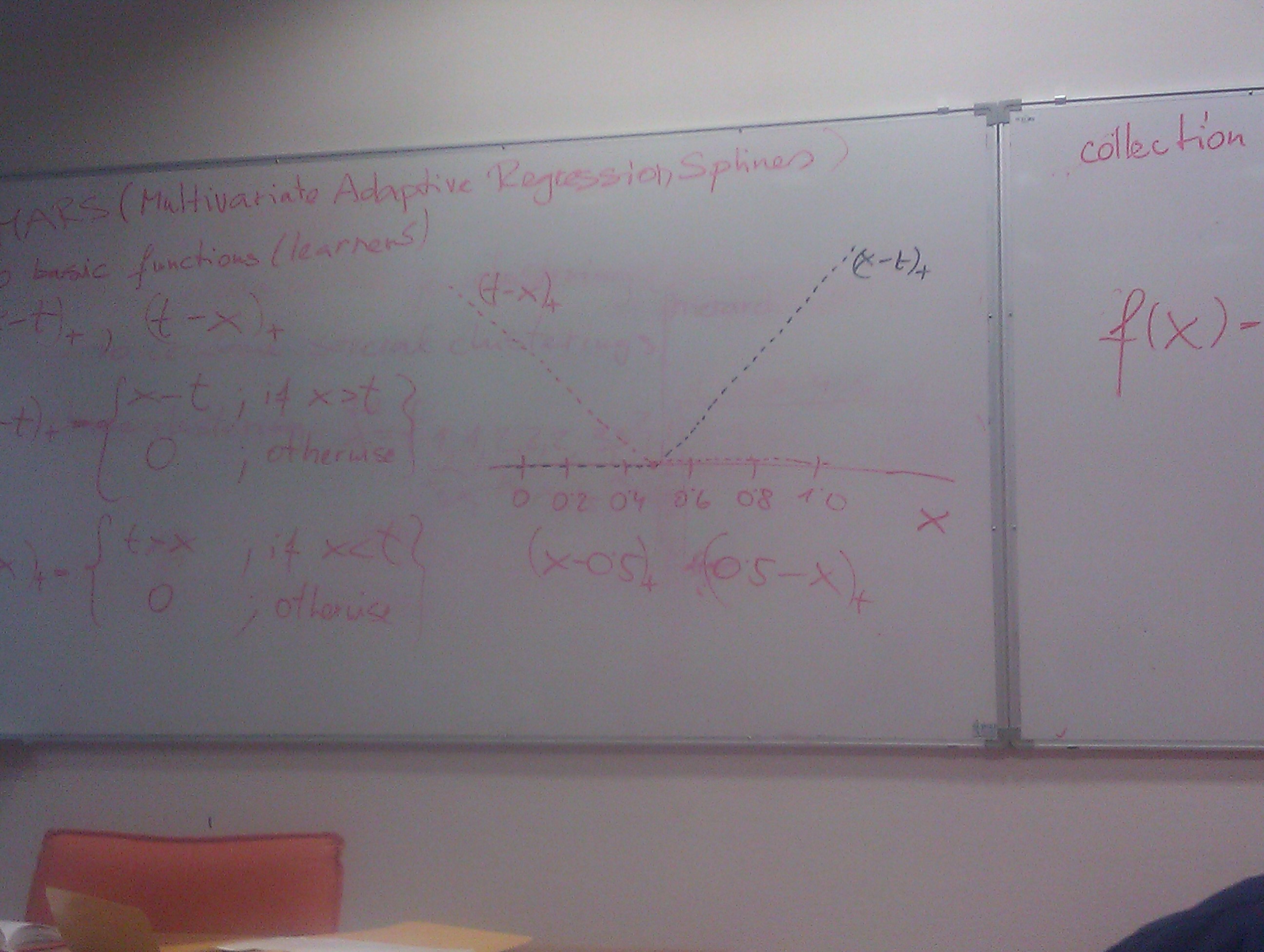
\[ (x-t)_+ = \begin{cases} x-t & \text{if } x > t \\ 0 & \text{else} \end{cases} \]

\[ (t-x)_+ = \begin{cases} t-x & \text{if } x < t \\ 0 & \text{else} \end{cases} \]

We put two such functions for \(t\) in every value of every attribute and than we want to combine them into an ensemble. We combine all by selecting only the useful ones. We multiply basic functions together.

Idea:

• collection \(C = \{(x_j-t)_+, (t-x_j)_+; t \in \{x_{1j}, x_{2j},...x_{nj}\}; j \in \{1,2,...a\}\}\)
• \(f(x) = \beta_0 + \sum_{m=1}^{M} \beta_m h_m(x)\)
• \(h_m(x) \in C\)
• effectively we multiply all collections \(C \times C \times ...C^i\)
• \(\beta_m\) – learn coefficients learn a generalized linear model (using least squares criterion)
• candidates consist of pairs of functions for each attribute value
• by multiplying more and more line segments we approximate the target function more and more
• we’ll probably over-fit it

Pseudo-code (iteratively create an ensemble members):

• start with a constant (\(1\))
• repeat until (satisfied)
• select best candidate multiplied with existing members
• add to model
• prune the model (using regularization or heuristic based on complexity)

Const-sensitive learning ensembles

Misclassification cost is the cost when we make an error. Represented as values in a matrix between predicted and actual classifications. Asymmetric misclassification cost matrix introduces cost-sensitive learning.

One re-sampling approach is done in boosting-type of algorithms where we push instances of high cost to classifiers.

Algorithm: MetaCost (based on bagging)

Input:

• training data \(D\)
• cost matrix \(C\), \(c_{ij}\) is the cost of misclassifying instance of class \(i\) as class \(j\)

Pseudo-code:

for(i=1 to T) {  // T number of basic models
  D_i = subsample of D with n instances (bootstrap)
  M_i = L(D_i)
  for(each x in D) {
    for(each class j) {
      P(j|x) = 1/T * sum_{i=1}^{T} (P(j|x,M_i))
    }
  }
  assign a label to x as: arg min_{i \in \{1,...c\}} sum_{j \in \{1,...c\}} P(j|x)*C_{ji} (we weight all probabilities by their cost)
}

Output:

• \(L(\{\text{a new dataset of }(x, \text{assigned class values})\})\)

Unbalanced dataset is where instances of one class are more probable than the other (eg. 1: 1%; 0: 99%). One possible approach is to use a cost matrix. Learning such data can result in overfitting.

Two approaches:

• oversampling
  • technique SMOTE: compute some neighborhood an linearly in between the instances of different classes create new instances, put them based on previous clustering, density
• undersampling (throw away some data)
  • search for instances near the border, other can be thrown away (similar to support vectors)

Algorithm: EasyEnsemble

Ideas is to repeat the under-sampling enough times \(T \sim \frac{|N|}{|P|}\).

Input:

• dataset \(D\)
• minority class examples \(P \in D\) (positive, outliers, precious)
• majority class instances \(N \in D\) (negative)
• \(T\) – number of subsets from \(N\)

Pseudo-code:

for(i=1 to T) {
  find a random subset N_i \in N with |N_i| = |P|
  use N_i and P to train AdaBoost ensemble H_i(x) = sign \sum_{j=1}^{S_i} a_{ij} * h_{ij}(x)
}

Output:

• \(H(x) = \operatorname{sign} \sum_{i=1}^{T} H_i(x)\)